
Deep Learning深度学习-学习笔记
This notes’ content are all based on https://www.coursera.org/specializations/deep-learning
Latex may have some issues when displaying.
1. Neural Networks and Deep Learning
1.1 Introduction to Deep Learning
1.1.1 Supervised Learning with Deep Learning
- Structured Data: Charts.
- Unstructured Data: Audio, Image, Text.
1.1.2 Scale drives deep learning progress
- The larger the amount of data, the better the performance of the larger neural network compare to smaller one or supervised learning.
- Sigmoid change to ReLU will make gradient descent much more faster. Since the gradient will not go to 0 really fast.
1.2 Basics of Neural Network Programming
1.2.1 Binary Classification
- Input:
- Output: 0, 1
1.2.2 Logistic Regression
Given , want
Input:
Parameters:
Output
- If large,
- If large negative number,
Loss (error) function:
- , where
Want
- If <- want as large as possible, want large
- If <- want as large as possible, want small
- , where
Cost function
1.2.3 Gradient Descent
- Repeat ;
- : Learning rate
- Right side of minimum, ; Left side of minimum,
- Logistic Regression Gradient Descent
- -->-->
- ()
- Gradient Descent on examples
- for to
- (for n = 2)
- (for n = 2)
- for to
1.2.4 Computational Graph
- Left to right computation
Derivatives with a Computation Graph
- Chain Rule:
1.2.5 Vectorization
avoid explicit for-loops.
- for to
- for to
- ; b(1,1)-->Broodcasting
Vectorization Logistic Regression
- Get rid of and in for loop
- New Form of Logistic Regression
Broadcasting(same as bsxfun in Matlab/Octave)
- +-\*/->1->m will be all the same number.
- +-\*/->1->n will be all the same number
- Don’t use “rank 1 array”
- Use or
- Check by
- Fix rank 1 array by
Logistic Regression Cost Function
- Lost
- If :
- If :
- Cost
- Use maximum likelihood estimation(MLE)
- Cost(minmize):
- Lost
1.3 Shallow Neural Networks
1.3.1 Neural Network Representation
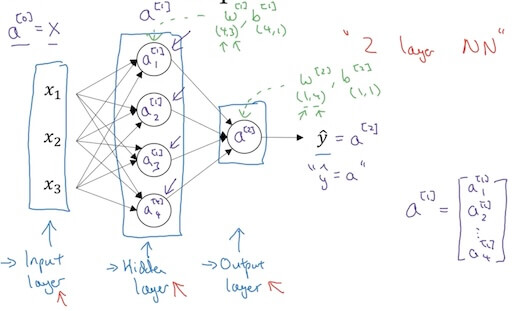
Input layer, hidden layer, output layer
- -> ->
- Layers count by # of hidden layer+# of output layer.
- -> ->
- First hidden node:
- Seconde hidden node:
- Third hidden node:
- Forth hidden node:
Vectorization
- : layer ; example
for i=1 to m:
Vectorizing of the above for loop
- n is different hidden units
- hrizontally: training examples; vertically: hidden units
1.3.2 Activation Functions
- : activation function of layer
- Sigmoid:
- Tanh:
- ReLU:
- Leaky ReLu:
- Rules to choose activation function
- Output is between {0, 1}, choose sigmoid.
- Default choose ReLu.
- Why need non-liner activation function
- Use linear hidden layer will be useless to have multiple hidden layers. It will become .
- Linear may sometime use at output layer but with non-linear at hidden layers.
1.3.3 Forward and Backward Propogation
- Derivative of activation function
- Sigmoid:
- Tanh:
- ReLU:
- Leaky ReLU:
- Gradient descent for neural networks
- Parameters:
- Cost function:
- Forward propagation:
- Back Propogation:
- Random Initialization
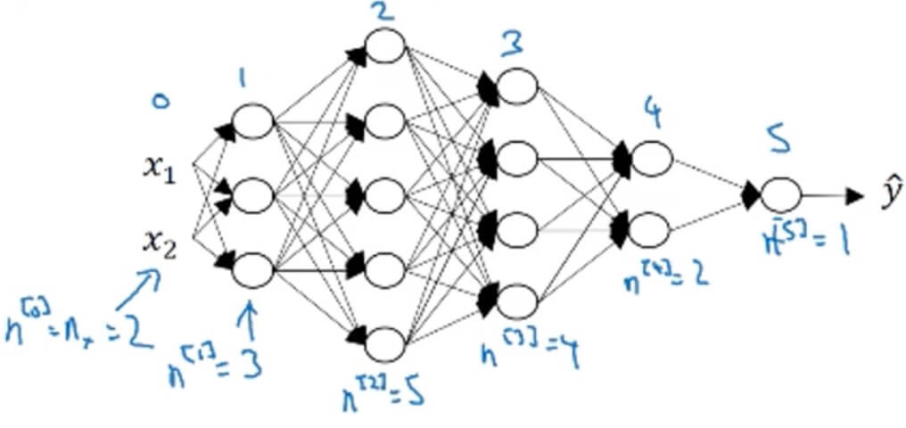
1.4 Deep Neural Networks
1.4.1 Deep L-Layer Neural Network
- Deep neural network notation
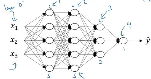
- (#layers)
1.4.2 Forward Propagation in a Deep Network
- General:
- …
- Vectorizing:
- Matrix dimensions
- Why deep representation?
- Earier layers learn simple features; later deeper layers put together to detect more complex things.
- Circuit theory and deep learning: Informally: There are functions you can compute with a “small” L-layer deep neural network that shallower networks require exponentially more hidden units to compute.
1.4.3 Building Blocks of Deep Neural Networks
- Forward and backward functions
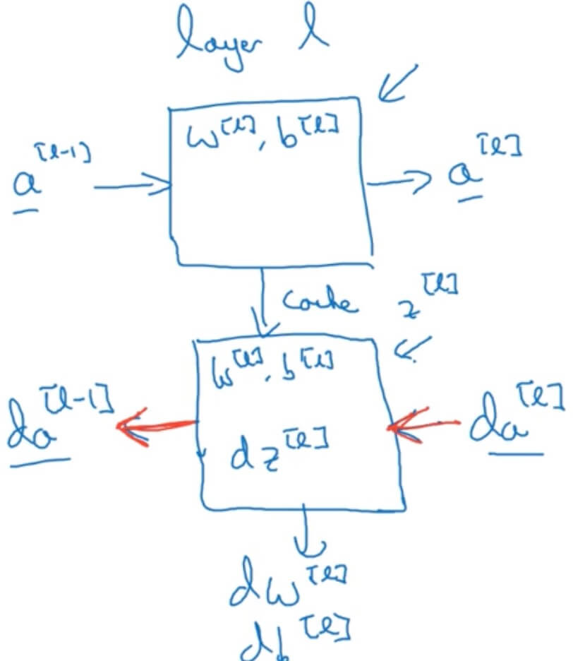
- Layer
- Forward: Input , output
- Backward: Input , output
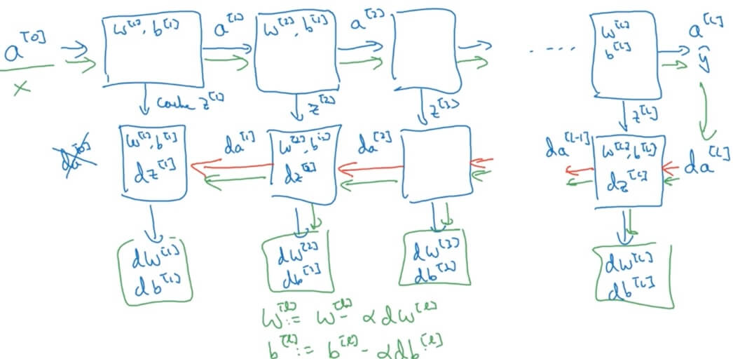
- One iteration of gradient descent of neural network
- How to implement?
- Forward propagation for layer
- Input , output
- Vectoried
- Backward propagation for layer
- Input , output
- Vectorized:
- Input , output
- Forward propagation for layer
1.4.4 Parameters vs. Hyperparameters
- Parameters:
- Hyperparameters (will affect/control/determine parameters):
- learning rate
- # iterations
- # of hidden units
- # of hidden layers
- Choice of activation function
- Later: momemtum, minibatch size, regularization parameters,…
II. Improving Deep Neural Networks: Hyperparameter Tuning, Regularization and Optimization
2.1 Practical Aspects of Deep Learning
2.1.1 Train / Dev / Test sets
- Big data may need only 1% or even less dev/test sets.
- Mismatched: Make sure dev/test come from same distribution
- Not having a test set might be okay. (Only dev set.)
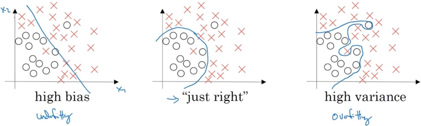
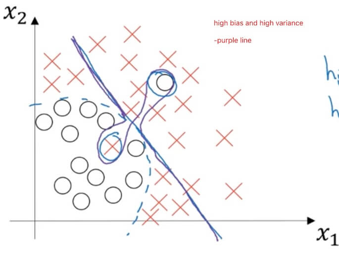
2.1.2 Bias / Variance
- Assume optimal (Bayes) error:
- High bias (underfitting): The prediction cannot classify different elemets as we want.
- Training set error , Dev set error .
- Training set error , Dev set error .
- “just right”: The prediction perfectly classify different elemets as we want.
- Training set error , Dev set error .
- High variance (overfitting): The prediction 100% classify different elemets.
- Training set error , Dev set error .
- Training set error , Dev set error .
2.1.3 Basic Recipe for Machine Learning
2.1.3.1 Basic Recipe
- High bias(training data performance)
- Bigger network
- Train longer
- (NN architecture search)
- High variance (dev set performance)
- More data
- Regulairzation
- (NN architecture search)
2.1.3.2 Regularization
- Logistic regression.
- L2 regularization
- L1 regularization
- will be spouse(for L1) (will have lots of 0 in it, only help a little bit)
- Neural network
- Frobenius norm: Square root of square sum of all elements in a matrix.
- (keep the same)
- Weight decay
-
-
- How does regularization prevent overfitting: bigger smaller smaller, which will make the activation function nearly linear(take tanh as an example). This will cause the network really hard to draw boundary with curve.
- Dropout regularization
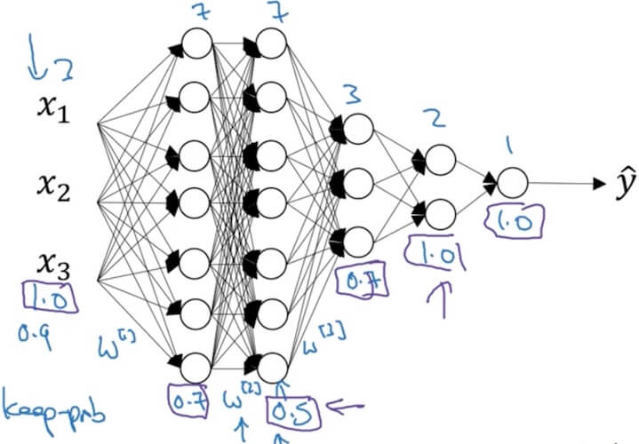
- Implementing dropout(“Inverted dropout”)
- Illustrate with layer (means 0.2 chance get dropout/be 0 out)
- #This will set d3 to be a same shape matrix as a3 with True (1), False (0) value.
- #a3\*=d3; This will let some neruons been dropout
- #inverted dropout, keep the total avtivation the same before and after dropout.
- Why work: Can’t rely on any one feature, so have to spread out weights.(shrink weights)
- First make sure the J is decreasing during iteration, then turn on dropout.
- Data augmentation
- Image: crop, flop, twist…
- Early stopping
- Mid-size
- May caused optimize cost function and not overfir at the same time.
- Orthogonalization
- Only consider optimize cost function or consider not overfit at one time.
2.1.3.3 Setting up your optimization problem
- Normalizing training sets
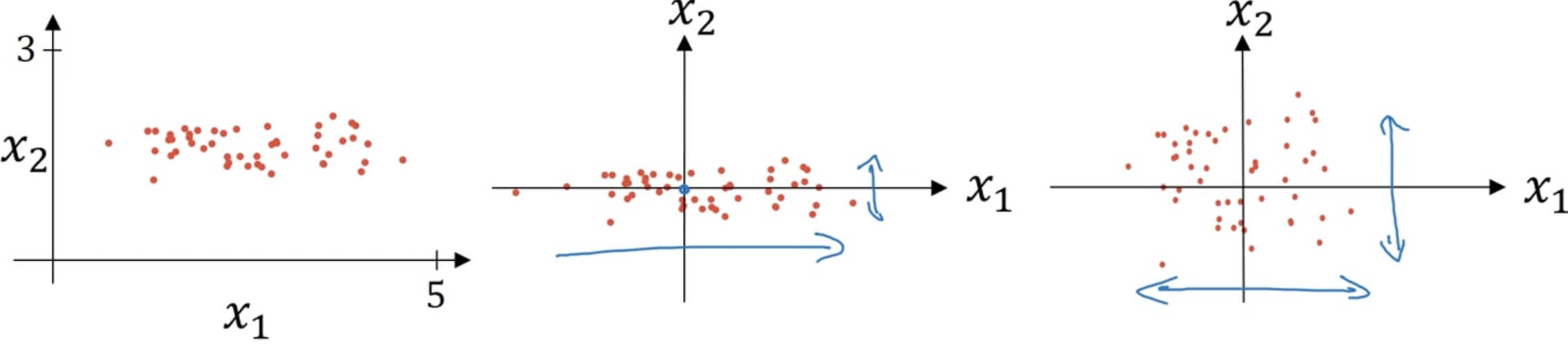
- Subtract mean:
- Normalize variance:
- "**" element-wise
- Use same to normalize test set.
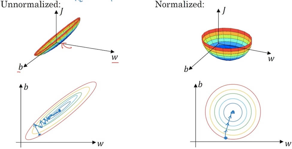
- Why normalize inputs?
- When inputs in very different scales will help a lot for performance and gradient descent/learning rate.
- Vanishing/exploding gradients
- Just slightly, will make the gradient increase really fast (exploding).
- Just slightly, will make the gradient decrease really slow (varnishing).
- Weight initalization (Single neuron)
- large (number of input features) –> smaller
- (sigmoid/tanh) ReLU: (variance can be a hyperparameter, DO NOT DO THAT)
- ReLU:
- Xavier initialization: Sometime
- Numerical approximation of gradients
- Gradient checking (Grad check)
- Take and reshape into a big vector .
- Take and reshape into a big vector .
- for each i:
- Check Euclidean distance (is Euclidean norm, sqare root of the sum of all elements’ power of 2)
- take , if above Euclidean distance is or smaller, is great.
- If is or bigger may need to check.
- If is or bigger may need to worry, maybe a bug. Check which i approx is difference between the real value.
- notes:
- Don’t use in training - only to debug.
- If algorithm fails grad check, look at components to try to identify bug.
- Remember regularization. (include the )
- Doesn’t work with dropout. (since is random, implement without dropout)
- Run at random initialization; perhaps again after some training. (not work when )
2.2 Optimization Algorithms
2.2.1 Mini-batch gradient descent
- Batch vs. mini-batch gradient descent
- Normal batch may have large amount of data like millions of elements.
- set
- Mini-batches make 1,000 each.
- Mini-batch number
- ith in trainning set, layer in network batch in mini-batch
- Mini-batch number
- Normal batch may have large amount of data like millions of elements.
- Mini-batch gradient descent
- 1 step of gradient descent using (1000)
- 1 epoch: single pass through training set.
- Forward prop on
- …
- Compute cost
- --> from
- Backprop to compute gradient cost
- 1 step of gradient descent using (1000)
- Understanding mini-batch gradient descent
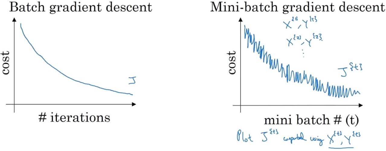
- If mini-batch size=m:batch gradient descent (Too long per iteration).–
- If mini-batch size=1:Stochatic gradient descent (noisy, not converge, loos speedup from vectorization).– Every example is it own mini-batch.
- In practice: select in-between 1 and m.
- Get lots of vectorization
- Make progress without needing to wait entire training set.
- Choosing mini-batch size
- No need for small training set ()
- Typical mini-batch size: 64, 128, 256, 512. (Use power of 2)
- Make sure minibatch fir in CPU/GPU memory.
2.2.2 Exponentially weighted averages
- is the weighted average at time .
- is the actual observed value at time .
- is the decay rate (usually between 0 and 1).
- is the weighted average at the previous time step.
Impact of Decay Rate : The value of significantly affects the smoothness of the weighted average curve:
- A larger makes the curve smoother, as it gives more weight to past observations, thereby reducing the impact of recent changes on the weighted average.
- A smaller makes the curve more responsive to recent changes, as it gives more weight to recent observations.
Interpretation of
- Defining as provides insight into how the influence of past data gradually diminishes as approaches 1 (i.e., approaches 0).
- As approaches 0, approaches , indicating that even though past data is given more weight (high ), its actual impact on the current value is decreasing.
Implementation
- Repear for each day:
- Get the next
Bias correction in exponentially weighted averages
- Bias correction is applied to counteract the initial bias in exponentially weighted averages, especially when the number of data points is small or at the start of the calculation.
- Here, is the uncorrected exponentially weighted average at time , and is the decay rate.
- It ensures that the moving averages are not underestimated, particularly when is high and in the early stages of the iteration. With iteration goes on, the affect of this correction will become smaller since is closer to 1.
Gradient descent with momentum
- On iteration t:
- Compute on current mini-batch (whole batch if not using mini-batch)
- initiate
- Smooth out gradient descent
- The momentum term effectively provides a smoothing effect since it is an average of past gradients. This means that extreme gradient changes in a single iteration are averaged out, reducing the volatility of the update steps.
- This smoothing effect is particularly useful on loss function surfaces that are not flat or have many local minima.
- Consider set as (common, about the average last 10 gradients), it gives more weight to , consider as the acceleration. With decreasing, velocity increasing slower and acceleration increasing faster.
- On iteration t:
2.2.3 RMSprop and Adam optimization
- RMSprop (Root Mean Square Propagation)
- On iteration t:
- Compute on current mini-batch
- Hope to be relative small.
- Hope to be relative large.
- is a realative small number() ot prevent nominaotr being 0.
- Slow down in vertical direction, fast in horizontal direction.
- On iteration t:
- Adam (Adaptive moment estimation) optimization algorithm
- On iteration t:
- Compute using current mini-batch
- Hyperparameters choice:
- : needs to be tune
- : 0.9 () First moment
- : 0.999 () Second moment
- Not affect performance
- Learning rate decay
- 1 epoch = 1 pass through the data
- Other methods
- ---- exponentially decay
- or ---- discrete staircase
- Manual decay (small number of model)
- The problem of local optima
- Unlikely to stuck in a bad local optima, since there are too many dimensions and all algorithms in deep learning.
- saddle point —- gradient = 0
- Problem of plateaus: Make learning slow
2.3.1 Tuning process
- Hyperparameters
- : learning rate (1st)
- : momentum (2nd)
- # of layers (3rd)
- # of hidden units (2nd)
- learning rate decay (3rd)
- mini-batch size (2nd)
- Try random values: Don’t use a grid
- Coarse to fine: Trying coarse random first, then fine in working well range.
2.3.2 Using an appropriate scale to pick hyperparameters
Learning rate:
- ----
- -----
- ----
Exponentially Weighted Averages Decay Rate:
- Reason for focusing on this instead of single : is too close to 1, small changes may have big affects.
In practice:
- Re-test/Re-evaluate occasionally.
- Babysitting one model (don’t have enough training capacity) (Panda): One model at one time.
- Training many models in parallel (Caviar): Can try many at same time.
2.3.3 Batch Normalization
- Implementing Batch Norm
- Batch Norm: make sure hidden units have standardized mean and variance.
- Given some intermediate value in NN (for some hidden layers, for 1 through )
- (Mean)
- (Variance)
- (Make sure mean=0, variance=1. prevent denominator=0)
- (are learnable parameters of model)
- If
- Then
- If
- Use instead of
- Adding Batch Norm to a network
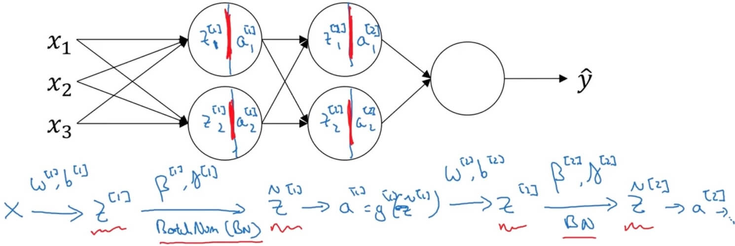
- Parameters:
- May use gradient/Adam/momentum to tune
- Working with mini-batches: Work the same but on single batches. No need for , since variance are all 1. have same dimension with .
- Implementing gradient descent (works with momentum, RMSprop, Adam)
- for …numMiniBatches
- Compute forwardProp on X^.
- In each hidden layer use BN to replace with
- Use backprop to compute (no )
- Update parameters
- Compute forwardProp on X^.
- for …numMiniBatches
- Why does Batch Norm work
- Covariate Shift: Different test and training data (training on black cats but try to test on other color of cats).
- Internal Covariate Shift: Between different layers of the network, the distribution of inputs to each layer changes. Recursively it changes the input of the latter layer. May lead to instability and reduced efficiency.
- Batch norm reduces the problem of input values changes. Make input stable. Let the network learn more independent.
- Batch norm as regularization
- In mini-batch, each batch is scaled by the mean/variance computed on just that mini-batch. May adds some noise to each hidden layer’s (since is not consider the whole training set) (similar to dropout).
- This has a slight regularization effect. (Use larger mini-batch size could reduce regularization)
- Covariate Shift: Different test and training data (training on black cats but try to test on other color of cats).
- Batch Norm at test time
- : estimate using exponentially weighted average (across mini-batch).
- During testing, use the global mean and variance estimates for normalization, instead of the statistics from the current test sample or mini-batch.
- : estimate using exponentially weighted average (across mini-batch).
2.3.4 Multi-class classification
- Softmax regression
- = # classes = 4 (0,...,3)
- Output layer: 4 nodes for each class. is (4,1) matrix, sum should be 1.
- (4,1) vector (L represents the output layer)
- Activation function:
- (4,1) vector
- Hardmax: Change beigest to 1, rest all set to 0.
- Training a softmax classifier
- If , softmax reduces to logistic regression.
- Loss function:
- ->->(4,1)
- Backprop: (4,1)
- Deep Learning frameworks
- TensorFlow
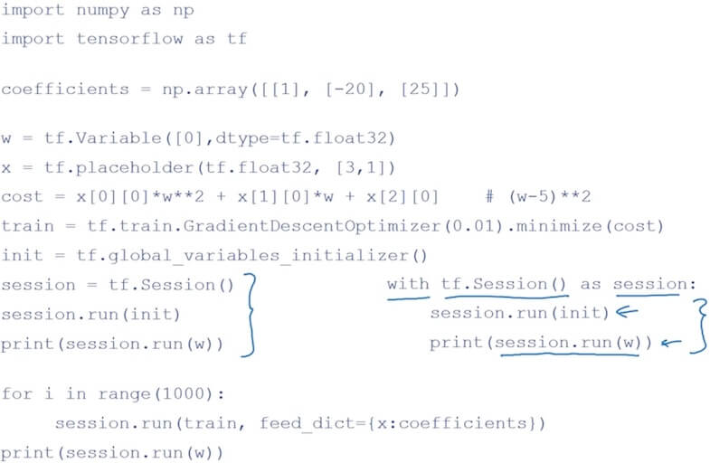
- TensorFlow
III. Structuring Machine Learning Projects
3.1 ML Strategy (1)
3.1.1 Setting up your goal
Orthogonalization
- Chain of assumptions in ML
- Fir training set well on cost function: bigger network; Adam
- Fit dev set well on cost function: Regularization; Bigger training set
- Fit test set well on cost function: Bigger dev set
- Perorms well in real world: Change dev set or cost function
- Chain of assumptions in ML
Single number evaluation metric
- Precision: In examples recognized, what percentage are actually true.
- Recall: What percentage of target are correctly recognized in whole test set.
- F1 Score: Average of precision and recall. (harmonic mean)
- Dev set + Single number evaluation matric: Speed up iteration
- Use average error rate instead of single error rate for each classes in estimate many classes at same time.
Satisficing and optimizing matrics
Consider classifiers with accuracy and running time.
- maximize accuracy and subject to running time <= 100ms
- Accuracy: optimizing
- Running time: satisfiying
N metic: 1 optimizing, n-1 satisficing
Train/dev/test distributions
- Come from same distribution. (Use randomly shuffle)
- Choose a dev set and test set to reflect data you expect to get in the future and consider important to do well on.
Size of dev/test set
- For large data set, use 98% training, 1% dev, 1% test
- Size of test set: Set your test set to be big enough to give high confidence in the overall performance of your system.
- Sometime use only train+dev, without test set.
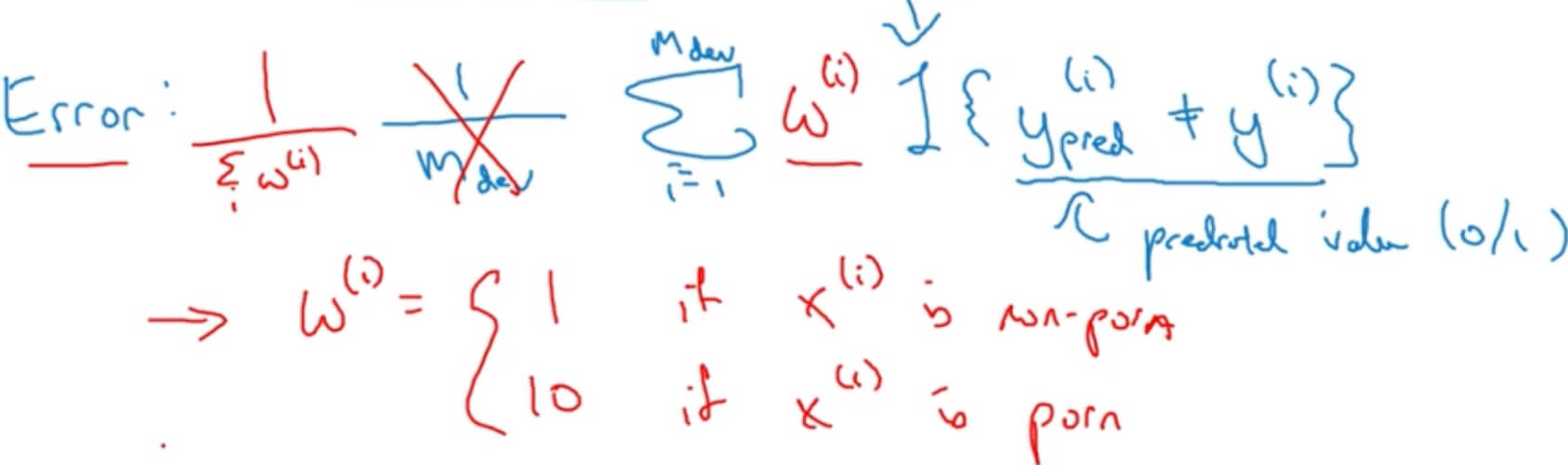
When to change dev/test sets and metrics
Filter pornographic images out of error rate:
Two Steps
- How to define a metric to evaluate classifiers.
- How to do well on this metric.
If doing well on your metric + dev/test set does not correspond to doing well on your application, change your metric and/or dev/test set.
3.1.2 Comparing to human-level performance
- Why human-level performance:
- Bayes (optimal) error: best possible error. Can never surpass.
- Humans are quite good at a lot of tasks. So long as ML is worse than humans, you can:
- Get labeled data from humans.
- Gain insight from manual error analysis: Why did a person get this right?
- Better analysis of bias/variance.
3.1.3 Analyzing bias and variance
- Avoidable bias
- If training error is far from human error (bayes error), focus on bias (avoidable bias). If training error is close to human error but far from dev error, focus on variance.
- Consider human-level error as a proxy for Bayes error (since is not too far from human-level error to Bayes error).
- Understanding human-level performance:
- Based on purpose defined which is the human-level error want to use.
- If human can perform really well, we can use human-level error as proxy for Bayes error.
- Surpassing human-level performance
- Not natural perception
- Lots of data
- Improving your model performance
- The two fundamental assumptions of supervised learning
- You can fit the training set pretty well. (Avoidable bias)
- The training set performance generalizes pretty well to the dev/test set. (Variance)
- Reducing (avoidable) bias and variance
- Avoidable bias:
- Train bigger model.
- Train longer/better optimization, algorithms (momentum, RMSprop, Adam).
- NN architecture/hyperparameters search (RNN, CNN).
- Variance:
- More data.
- Regularization (L2, dropout, data augmentation).
- NN architecture/hyperparameters search.
- Avoidable bias:
- The two fundamental assumptions of supervised learning
3.2 ML Strategy (2)
3.2.1 Error analysis
- Carrying out error analysis
- Error analysis (count mislabel, minus from the error rate get the ceiling of error rate)
- Get ~100 mislabeled dev set examples.
- Count up how many are dogs.
- Evaluate multiple ideas in parallel (ideas for cat detection)
- Fix pictures of dogs being recognized as cats
- Fix great cats (lions, panthers, etc.) being misrecognized
- Improve performance on blurry images
- Check the details of mislabeled images (only few minutes/hours)
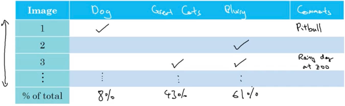
- Error analysis (count mislabel, minus from the error rate get the ceiling of error rate)
- Cleaning up incorrectly labeled data
- DL algorithms are quite robust to random errors in the training set. (random error will not affect the algorithm too much)
- DL algorithms are less robust to systematic errors.
- When a high fraction of mistake is due to incorrectly label, should spend time to fix it.
- Correcting incorrect dev/test set examples
- Apply same process to your dev and test sets to make sure they continue to come from the same distribution.
- Consider examining examples your algorithm got right as well as ones it got wrong.
- Train and dev/test data may now come from slightly different distributions.
- Build your first system quickly, then iterate
- Set up dev/test set and metric
- Build initial system quickly
- Use Bias/Variance analysis & Error analysis to prioritize next steps.
- Training and testing on different distributions
- 200,000 from high quality webpages, 10,000 from low quality mobile app (but we care about this).
- Shuffle before use those data. (not a good option, will cause the influence of what we care small.)
- Use mobile app as dev/test set, and just really small part of training set from app. (This we will make our target to what we want.) Maybe 50% in training, 25% in dev, and 25% test.
- 200,000 from high quality webpages, 10,000 from low quality mobile app (but we care about this).
3.2.2 Mismatched training and dev/test set
- Training-dev set: Same distribution as training set, but not used for training.
- Training error - Training-dev error - Dev error
- Human level - traning set error: avoidable bias
- Traning error - Training-dev error: Variance
- Training-dev error - Dev error: Data mismatch
- Dev error - Test error: degree of overfitting to dev set.
- Addressing data mismatch
- Carry out manual error analysis to try to understand difference between training and dev/test sets.
- Make training data more similar; or collect more data similar to dev/test sets.
- Artificial data synthesis:
- Possible issue (overfitting): Original data is 10000, only have the noise of 1, maybe overfit to this 1.
- Transfer learning
- Pre-training/Fine-tune
- From relatively large data to relatively small data.
- But if the target data is too small may not be suitable for transfer learning. (Depend on the outcome we want, it would be valuable to have more data)
- When makes sense (transfer from A-> B):
- Task A and B have the same input x.
- You have a lot more data for Task A than Task B (want this one).
- Low level features from A could be helpful for learning B.
3.2.3 Learning from multiple tasks
- Loss function for multiple tasks
- Loss:
- Sum only over valid of j with 0/1 label. (some of them may only labeled some feature)
- Unlike softmax regression: One image can have multiple labels
- When multi-task learning makes sense
- Training on a set of tasks that could benefit from having shared lower-level features.
- Usually: Amount of data you have for each task is quite similar.
- Can train a big enough neural network to do well on all the tasks.
3.2.4 End-to-end deep learning
- End-to-end needs lots of data to work well.
- Breaking small data scenario into different deep learning will be better results.
- Wether to use end-to-end learning
- Pros:
- Let the data speak.
- Less hand-designing of components needed.
- Cons:
- May need large amount of data
- Excludes potentially useful hand-designed components.
- Key question: Do you have sufficient data to learn a function of the complexity needed to map x to y?
- Use DL to learn individual components.
- Carefully choose X->Y mappping depending on what tasks you can got data for.
- Pros:
IV. Convolutional Neural Networks
4.1 Foundations of Convolutional Neural Networks
4.1.1 Convolutional operatin
Vertical Edge Detection
- Used to identify vertical edges in images, which is a crucial step in image analysis and understanding.
- A small matrix, typically 3x3 or 5x5, is used as a convolution kernel to detect vertical edges.
- The kernel slides over the image, moving one pixel at a time.
- At each position, element-wise multiplication is performed between the kernel and the overlapping image area, followed by a sum to produce an output feature map.
- High values in the output feature map indicate the presence of a vertical edge at that location.
- $
\begin{bmatrix}
1 & 0 & -1 \
1 & 0 & -1 \
1 & 0 & -1
\end{bmatrix}
$ - Based on this matrix example below, it will detect lighter on the left and darker on the right.
Horizontal Edge Detection
- Brighter on the top and darker on the bottom
- $
\begin{bmatrix}
1 & 1 & 1 \
0 & 0 & 0 \
-1 & -1 & -1
\end{bmatrix}
$ - TBC
Other Common Filters
Sobel filter
- $
\begin{bmatrix}
1 & 0 & -1 \
2 & 0 & -2 \
1 & 0 & -1
\end{bmatrix}
$
- $
Scharr filter
- $
\begin{bmatrix}
3 & 0 & -3 \
10 & 0 & -10 \
3 & 0 & -3
\end{bmatrix}
$
- $
Padding
nxn * fxf = n-f+1 x n-f+1
Problems of convolution:
- Shrinking output
- Through away information from edge.
Add a padding(p) of 0
- n+2pxn+2p * fxf = n+2p-f+1 x n+2p-f+1
Valid convolutions: No padding
Same convolutions: Pad so that output size is the same as the input size. (padding is )
f is usually odd.
Strided convolution
- Stepping s steps instead of 1.
- x (If not integer, bound down to the nearest integer.)
cross-correlation is the real name of convolution in DL.
Convolution over volume
- Set the filter into the same volume as the input matrix. (e.g. RGB image with 3x3x3 filter)
- If only look at an individual channel, just make other channel with all 0.
- If consider vertical and horitental seperately, each output 4x4, the final could stack together get a 4x4x2 volume.
- -> (\# of filters)
One layer of a CNN
- Each output add a bias and apply non-learner to it. ReLU(Output+b) –> Consider stack all outputs after this as volume as the a in a=g(z)
- Consider output as the same as the w in z=wa+b.
- Number of parameters in one layer: If you have 10 filters that are 3x3x 3 in one layer of a neural network, how many parameters does that layer have?(Consider 3x3x3 + bias, it will be 280 parameters)
Summary of notation (If layer 1 is a convolution layer)
- filter size (3x3 filter will be f=3)
- padding
- stride
- Input:
- Output:
- Round down to nearest integer
- Each filter is:
- Activations: -> Batch gradient descent ->
- Weights: (The last quantity is # filters in layer l)
- bias: -
A simple example ConvNet
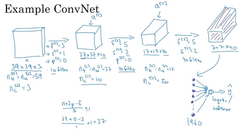
- Get the final output(7x7x40) and take it as a 1960 vector pass through logistic/softmax to get out actual final value.
Types of layer in a convolutional network
- Convolution (CONV)
- Pooling (POOL)
- Fully connected (FC)
4.1.2 Pooling layers
- No parameters to learn.
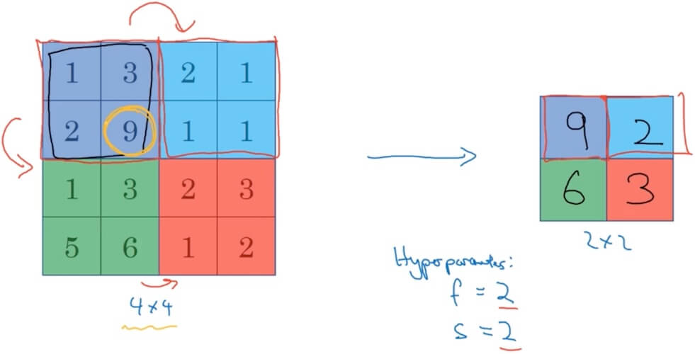
- Max pooling
- Consider input is 4x4 matrix, output a 2x2 matrix. f(filter) = 2, s(stride) = 2. Just max each 2x2 in the input and put it into one cell in the output matrix.
- Hyperparameters: f(filter) and s(stride).
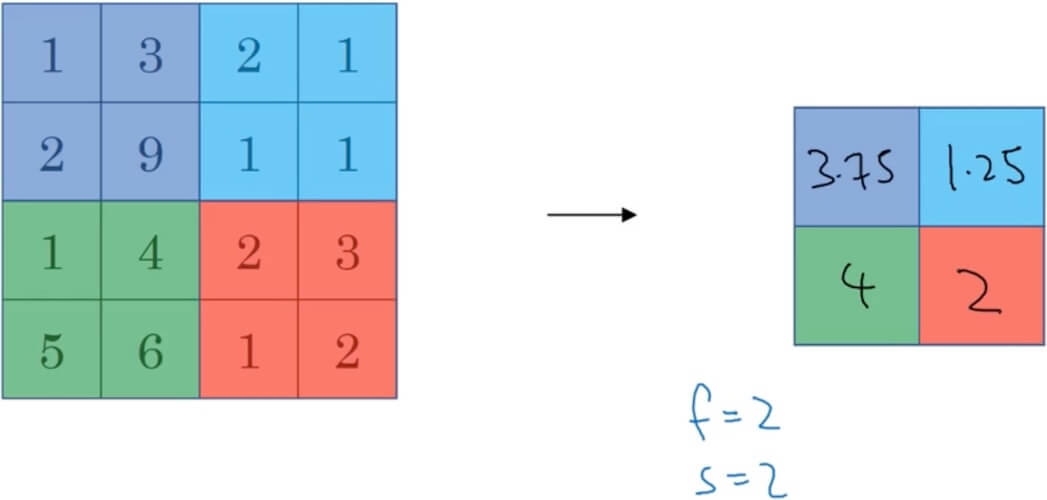
- Average pooling
- Instead of take the maxium, take the average.
- Input:
- Output: Down to the nearest integer.
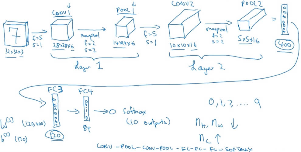
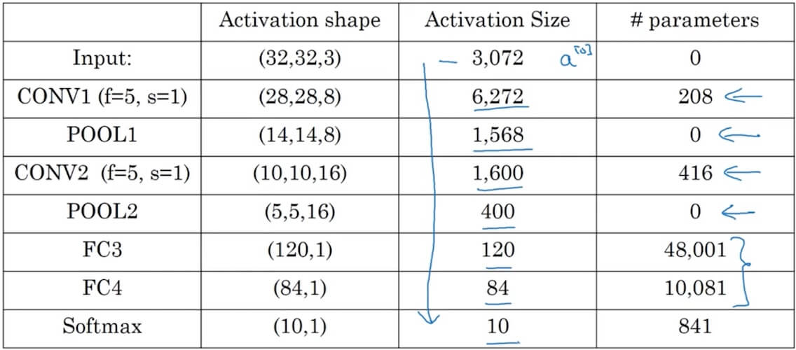
4.1.3 CNN example
- Fully Connected layer
- After several convolutional and pooling layers, the high-level reasoning in the neural network is done via FC layers. The output of the last pooling or convolutional layer, which is typically a multi-dimensional array, is flattened into a single vector of values. This vector is then fed into one or more FC layers.
- Role:
- Integration of Learned Features: FC layers combine all the features learned by previous convolutional layers across the entire image. While convolutional layers are good at identifying features in local areas of the input image, FC layers help in learning global patterns in the data.
- Dimensionality Reduction: FC layers can be seen as a form of dimensionality reduction, where the high-level, spatially hierarchical features extracted by the convolutional layers are compacted into a form where predictions can be made.
- Classification or Regression: In classification tasks, the final FC layer typically has as many neurons as the number of classes, with a softmax activation function being applied to the output. For regression tasks, the final FC layer’s output size and activation function are adjusted according to the specific requirements of the task.
- Operation is similar to neurons in a standard neural network.
- Example
- Why convolutions?
- Parameter sharing: A feature detector (such as a vertical edge detector) that’s useful in one part of the image is probably useful in another part of the image.
- Sparsity of connections: In each layer, each output value depends only on a small number of inputs.
- Training set
- Cost
4.2 Deep Convolutional Models: Case Studies
4.2.1 Case studies (LeNet-5, AlexNet, VGG, ResNets)
- Red notations in the image below are what the network original designed but not suitable for nowadays.
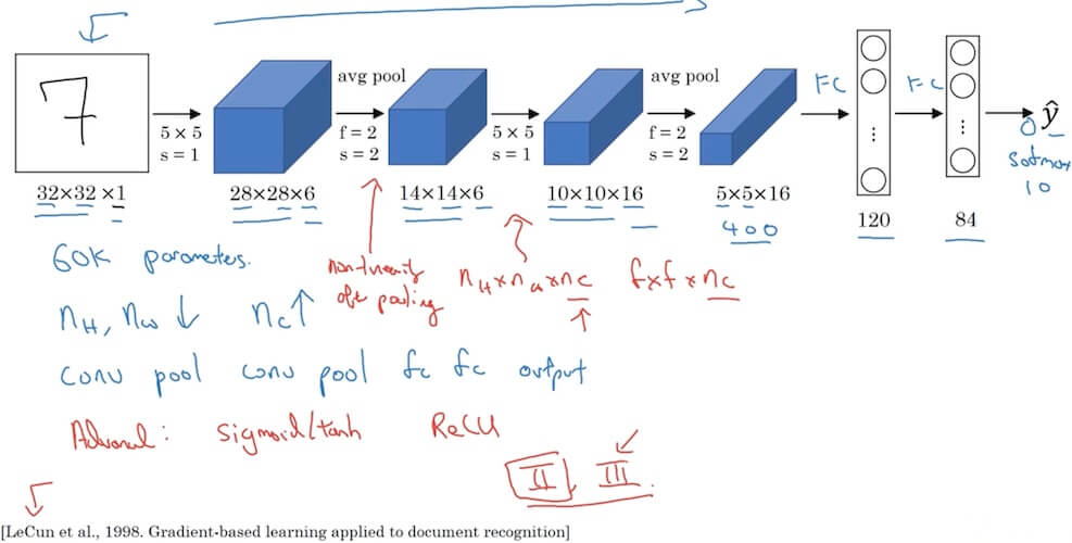
4.2.1.1 LeNet-5
- Pioneer in CNNs: One of the earliest Convolutional Neural Networks, primarily used for digit recognition tasks.
- Architecture:
- Consists of 7 layers (excluding input).
- Includes convolutional layers, average pooling layers, and fully connected layers.
- Activation Functions: Uses sigmoid and tanh activation functions in different layers. (Not using nowadays)
- Local Receptive Fields: Utilizes 5x5 convolution filters to capture spatial features.
- Subsampling Layers: Employs average pooling for subsampling. (Using max pool nowadays)
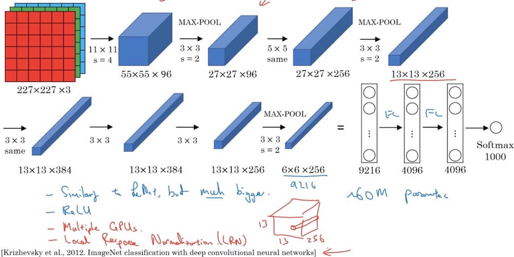
4.2.1.2 AlexNet
- Multiple GPUs in the paper is outdated for today. LRN is not useful after lots of other researches.
- Deeper Architecture: Contains 8 learned layers, 5 convolutional layers followed by 3 fully connected layers.
- ReLU Activation: One of the first CNNs to use ReLU (Rectified Linear Unit) activation function for faster training.
- Overlapping Pooling: Uses overlapping max pooling, reducing the network’s size and overfitting.
- Data Augmentation and Dropout: Employs data augmentation and dropout techniques for better generalization.
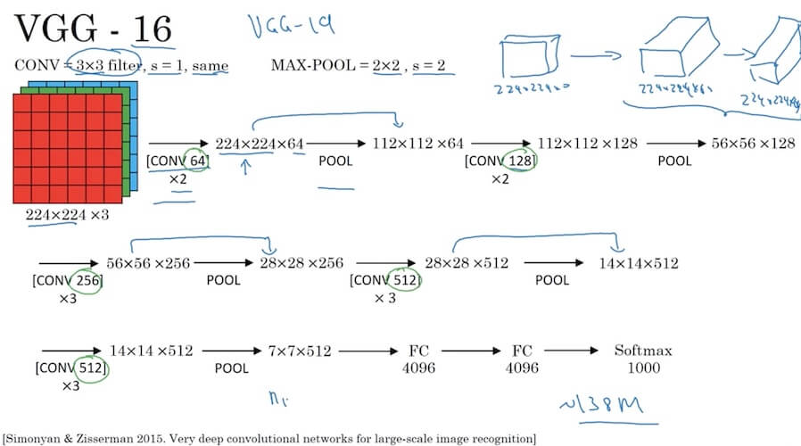
4.2.1.3 VGG-16
- Simplicity and Depth: Known for its simplicity and depth, with 16 learned layers.
- Uniform Architecture: Features a very uniform architecture, using 3x3 convolution filters with stride and pad of 1, max pooling, and fully connected layers.
- Convolutional Layers: Stacks convolutional layers (2-4 layers) before each max pooling layer.
- Large Number of Parameters: Has a high number of parameters (around 138 million), making it computationally intensive.
- Transfer Learning: Proved to be an excellent model for transfer learning due to its performance and simplicity.
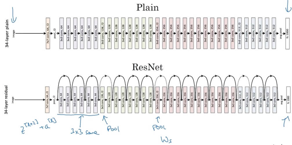
4.2.1.4 ResNets
Residual block
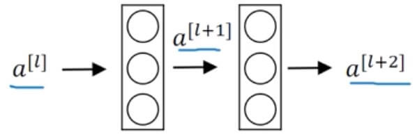
- Main Path: –> Linear –> ReLU –> –> Linear –> ReLU –>
- Short Cut / Skip Connection: –> ReLU –>
In normal plain network, the trainning error with increasing number of layers in theory will continuesly decrease. But in reality it will decrease but increase after a sweet point. What ResNet performs is decreasing training error with numbers of layers increase and the training error not increasing again.
Why do residual networks work?
Residual networks introduce a shortcut or skip connection that allows the network to learn identity functions effectively.
This is crucial for training very deep networks by avoiding the vanishing gradient problem.
In a residual block:
- -> BigNN -> -> Residual block ->
- Input is passed through a standard neural network (BigNN) to obtain , and then it goes through the residual block to produce .
- The formulation of a residual block can be represented as:
- Here, is the activation function.
- is the output of the layer just before the activation function.
- and are the weight and bias of the layer, respectively.
- If and , then , effectively allowing the network to learn the identity function.
- In cases where the dimensions of and differ (e.g., and ), a linear transformation (e.g., ) is applied to to match the dimensions.
This architecture enables training deeper models without performance degradation, which was a significant challenge in deep learning before the development of ResNet.
Understand through backdrop(personal notes not from the class content)
- Consider input as x, the residual block calculation as F(x), identity mapping just drag the x and add it to the residual block’s calculation which makes the final value
- Backprop for this will be as follow
- Gradient of the Residual Blokc’s Output:
- This represents the gradient of the output with respect to the weights .
- By chain rule:
- Since , and should be 1
- So the formula become
- Gradient of the Residual Blokc’s Output:
- Compare to without the identity mapping added. , there is a less. Add this to makes the network will not get worse results compare to before.
4.2.2 Network in Network and 1 X 1 convolutions
- 1x1 convolutions
- Functionality of 1x1 Convolutions: A 1x1 convolution, despite its simplicity, acts as a fully connected layer applied to each pixel separately across depth. It’s effectively used for channel-wise interactions and dimensionality reduction.
- Increasing Network Depth: 1x1 convolutions can increase the depth of the network without a significant increase in computational complexity.
- Dimensionality Reduction: They are often used for reducing the number of channels (depth) before applying expensive 3x3 or 5x5 convolutions, thus reducing the computational cost.
- Feature Re-calibration: 1x1 convolutions can recalibrate the feature maps channel-wise, enhancing the representational power of the network.
- Using 1x1 convolutions:
- Reduce dimension: Consider a 28x28x192 input with CONV 1x1 with 32 filters, the output will be 28x28x32.
4.2.3 Inception network
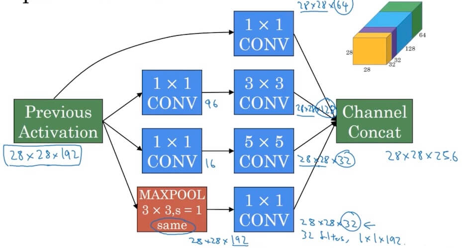
- Motivation for inception network
- Input 28x28x192
- Use 1x1x192 with 64 filters, output 28x28x64
- Use same dimension 3x3x192, output 28x28x128
- Use same dimension 5x5x192, output 28x28x32
- use same dimension and s=1 Max-Pool, output 28x28x32.
- Final output 28x28x256.
- The problem of computational cost (Consider 5x5x192)
- 5x5x192x28x28x32 is really big, 120M.
- Bottleneck layer (Using 1x1 convolution): shrink 28x28x192 –> CONV, 1x1, 16, 1x1x192 –> 28x28x16 (Bottleneck layer) –> CONV 5x5, 32, 5x5x16 –> 28x28x32
- In total only 28x28x16+28x28x32x5x5x16=12.4M
- Input 28x28x192
- Inception moule
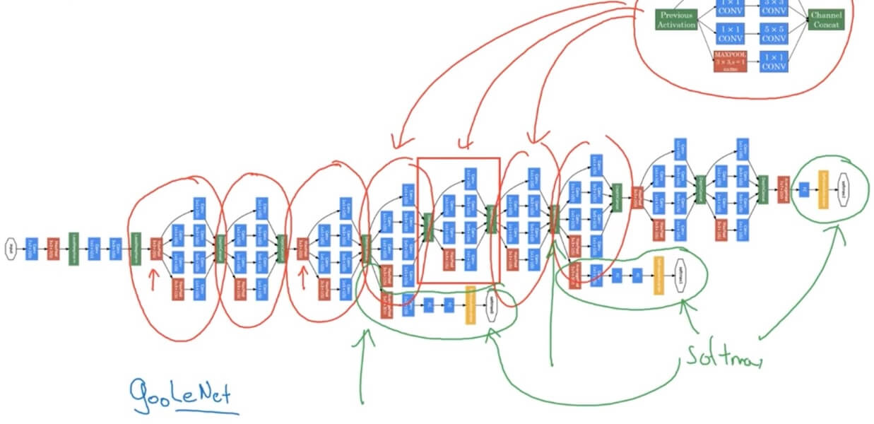
- The softmax in the itermediate position is used for regularization which is used avoid overfitting.
4.2.4 MobileNet
Depthwise Separable Convolution
- Depthwise Convolution
- Computational cost = #filter params x #filter positions x #of filters
- Ppointwise Convolution
- Computational cost = #filter params x #filter positions x # of filters
- Computational cost = #filter params x #filter positions x # of filters
- Cost of depthwise seprable convolution / normal convolution
- Depthwise Convolution
MobileNet v2 Bottleneck
Residual Connection
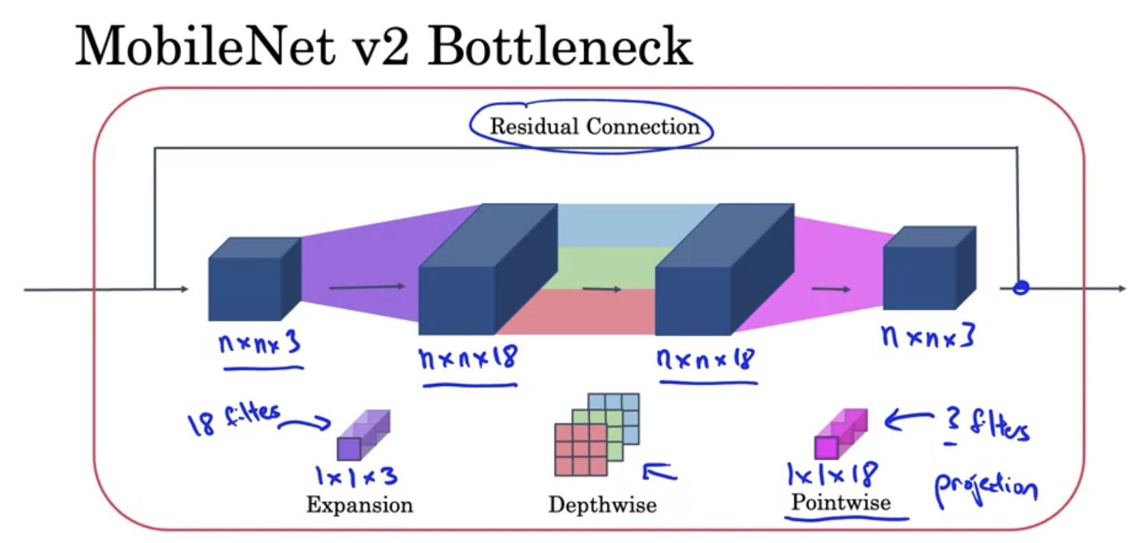
- Expansion
- Depthwise
- Pointwise (Projection)
Similar computational cost as v1
- MobileNet V2 improves upon V1 by introducing an inverted residual structure with linear bottlenecks, which enhances the efficiency of feature extraction and information flow through the network. This architectural advancement allows V2 to achieve better performance than V1, despite having similar computational costs. Essentially, V2 optimizes the way features are processed and combined, providing more effective and complex feature representation within the same computational budget as V1.
4.2.5 EfficientNet
- EfficientNet is a series of deep learning models known for high efficiency and accuracy in image classification tasks.
- Compound Scaling:
- It introduces a novel compound scaling method, scaling network depth, width, and resolution uniformly with a set of fixed coefficients.
- High Efficiency and Accuracy:
- EfficientNets provide state-of-the-art accuracy for image classification while being more computationally efficient compared to other models.
4.2.6 Inception network
- Transfer Learning
- Small training set: Freeze all hidden layers (save to disk), only train the softmax unit.
- Big training set: Freeze less hidden layers, train some of the hidden layers (or use new hidden units), and also own softmax unit.
- Lots of data: Use the already trained weights and bias as initalization, re-train based on it, as well as the softmax unit.
- Data augmentation
- Common augmentation method: Mirroring, Random Cropping, (Rotation, Shearing, Local warping, …)
- Color shifting: add/minus from RGB. Advanced: PCA / PCA color augmentation.
- Implementing distortions during training: One CPU thread doing augmentation, and other threads or GPU doing the training at same time.
- State of CV
- Data needed (little data to lots of data): Object detection < Image recognition < Speach recognition
- Lots of data - Simpler algotithms (Less hand-engineering)
- Little data - more hand-engineering (“hacks”) - Transfer learning
- Two sources of knowledge
- Labeled data
- Hand engineered features/network architecture/other components
- Tips for doing well on benchmarks/winning competitions
- Ensembling: Train several networks independently and average their outputs () 1-2% better. (3-15 networks)
- Multi-crop at test time: Run classifier on multiple versions of test images and average results. (10-crop: center, four corner, also on mirror image the same 5 crops)
- Use open source code
- Use architectures of networks published in the literature.
- Use open source implementations if possible.
- Use pretrained models and fine-tune on your dataset.
4.3 Object Detection
4.3.1 Object localization
- Want to detect 4 class: 1-pedestrian, 2-car, 3-mtorcycle, 4-background.
- Defining the target label y: Need to out put , class label (1-4). (In total 9 elements in the output vector).
- There is an object
- No object Don’t care for all of other
- Lost function:
- if
- if
4.3.2 Landmark detection
- Annotate key positions (points-xy coordinate) as landmarks.
4.3.3 Object detection
Object detection
- Starts with closely crops images.
- A window sliding from the top left to bottom right, once and once. If not find increase the window’s size and redo the sliding.
- Run each individual image to the convnet.
Turning FC layer into convolutional layers
- Instead directly to FC, use conv filter.
Convolution implementation of sliding windows
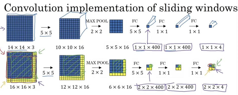
- Instead of do 4 times 14x14x3, new conv fc share the computation, directly using the 2x2x4.
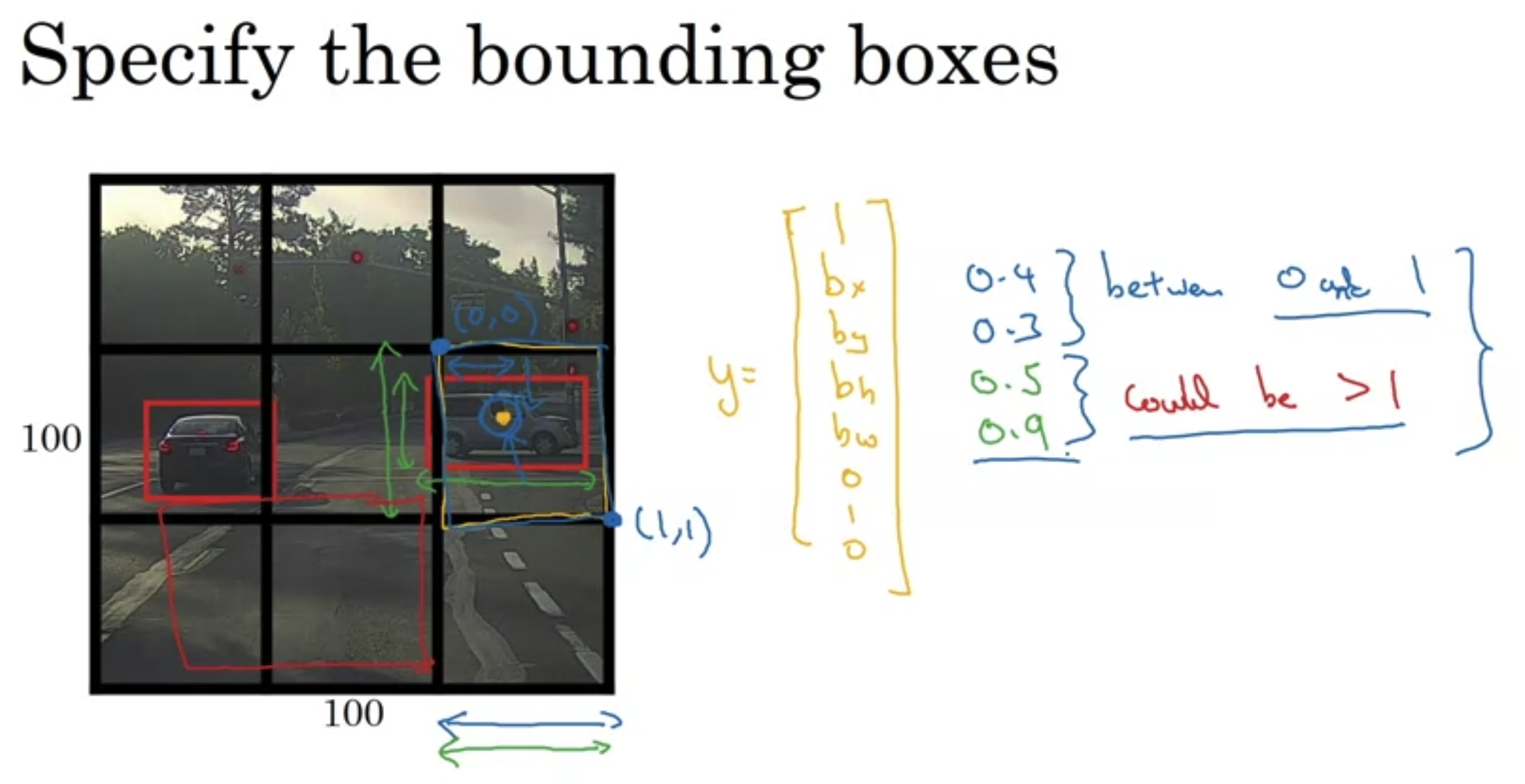
Output accurate bounding boxes
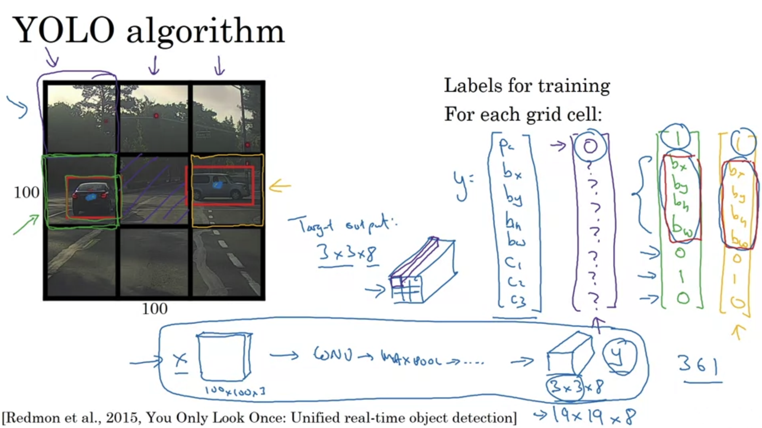
YOLO algorithm
- Find the medium point of target and working into the boundary box that contains that point.
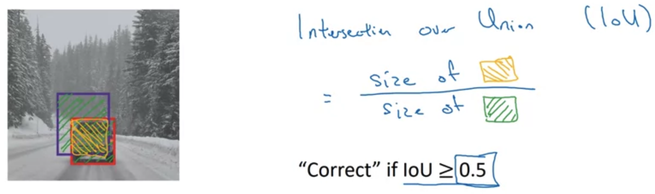
Intersection over union (IoU)
- Use to check accuracy.
- Size of intersection / size of reunion (normally “Correct” if loU 0.5)
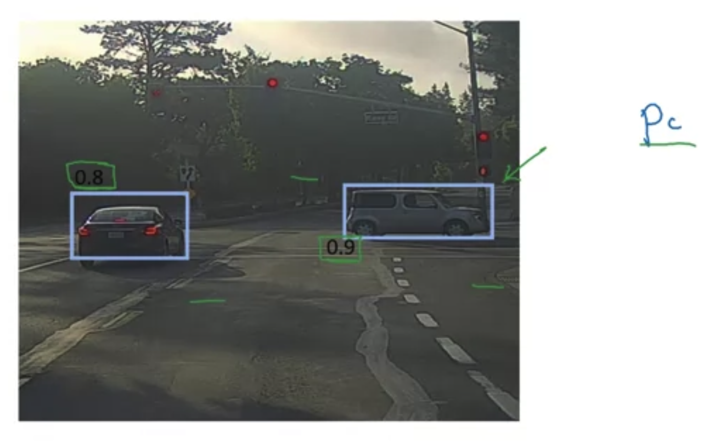
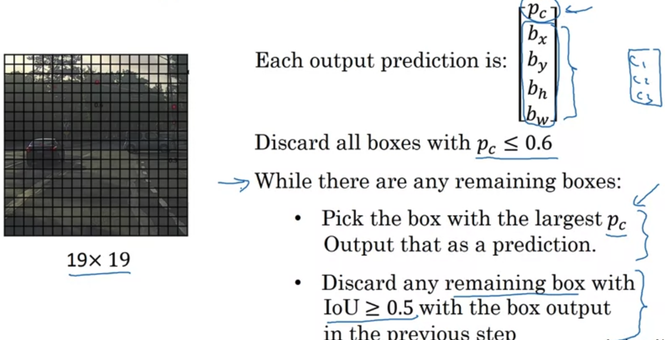
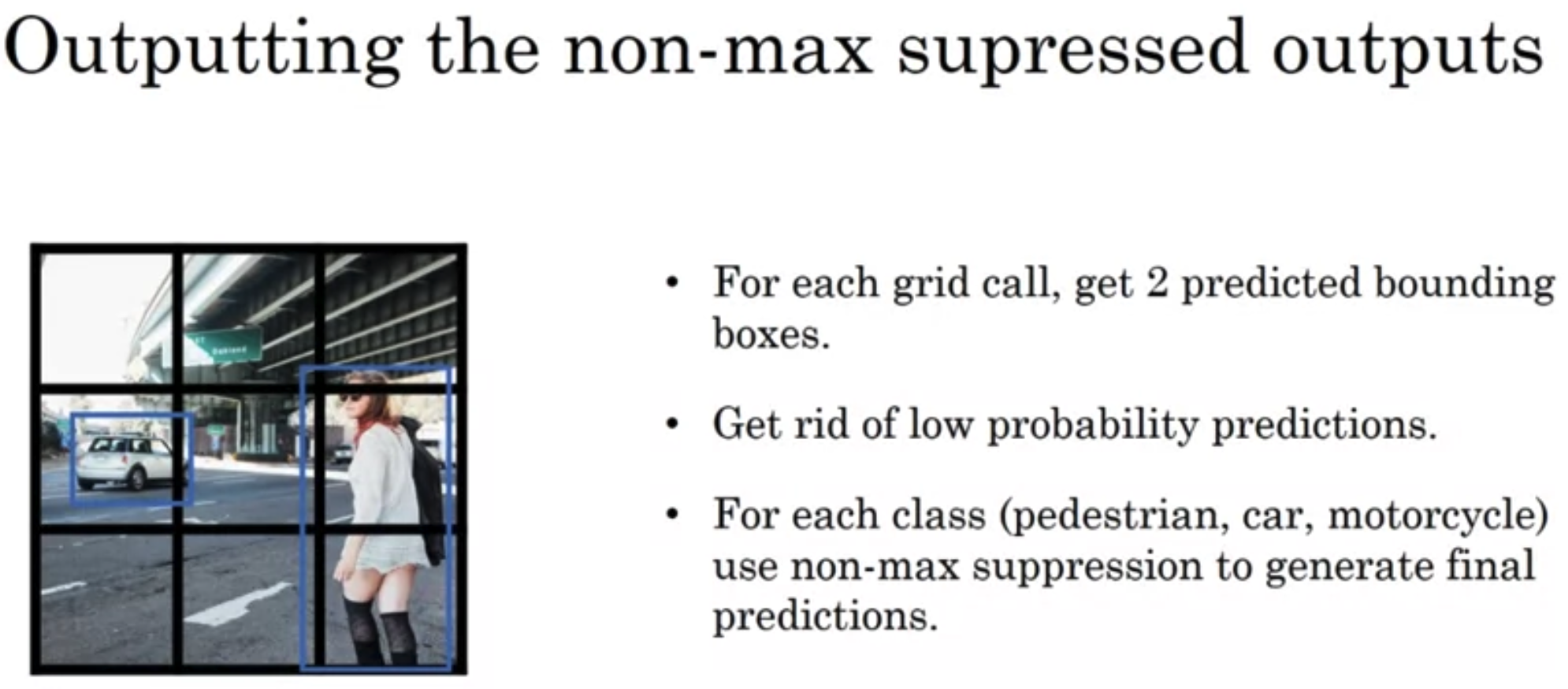
Non-max suppression
- Leave the maximum accuracy one, supprese all with high IoU.
Anchor Boxes
- Predefine anchor boxes, associate ojects with anchor boxes.
- If objects more than assigned anchor boxes, not works. Not same shape, not works.
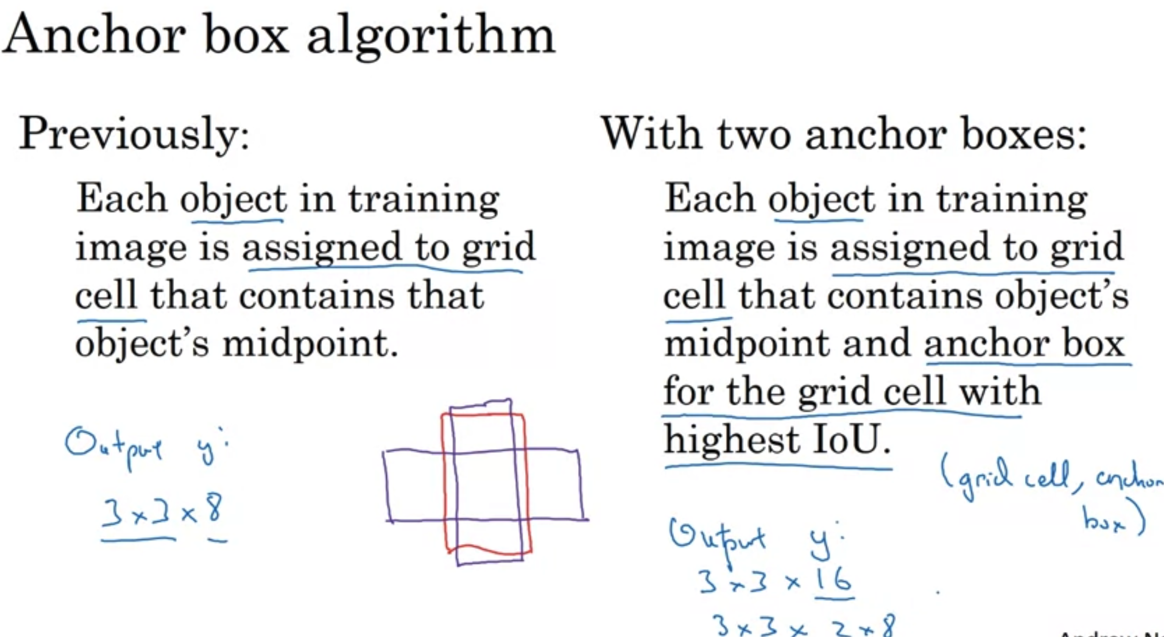
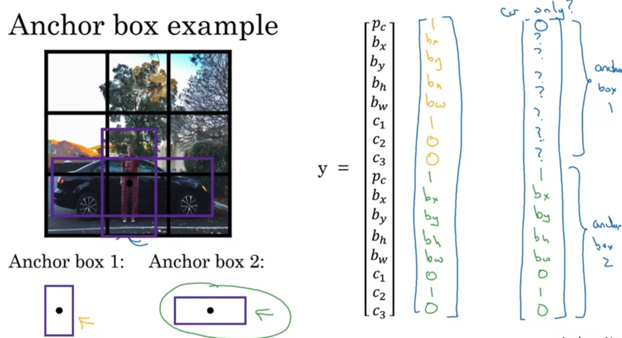
Training set
- y is 3x3x2x8 (which is # of grids x # of anchors x # classes(5() + classes))
Regision Proposals
- R-CNN: Propose regions. Classify proposed regions one at a time. Output label + bounding box.
- Fast R-CNN: Propose regions. Use convolution implementation of sliding windows to classify all the proposed regions.
- Faster R-CNN: Use convolutional network to propose regions.
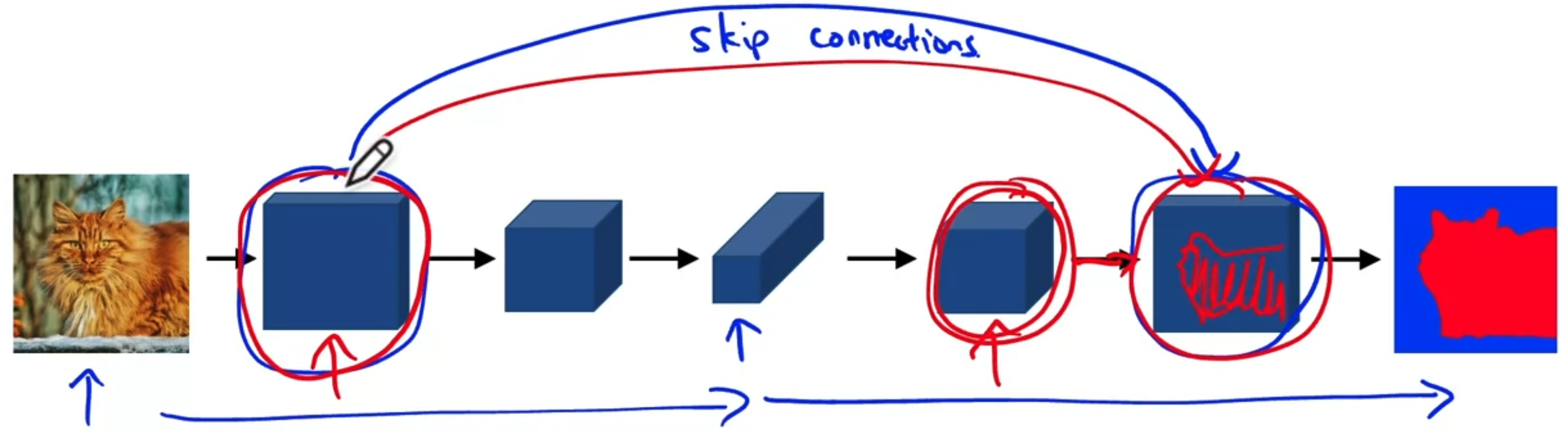
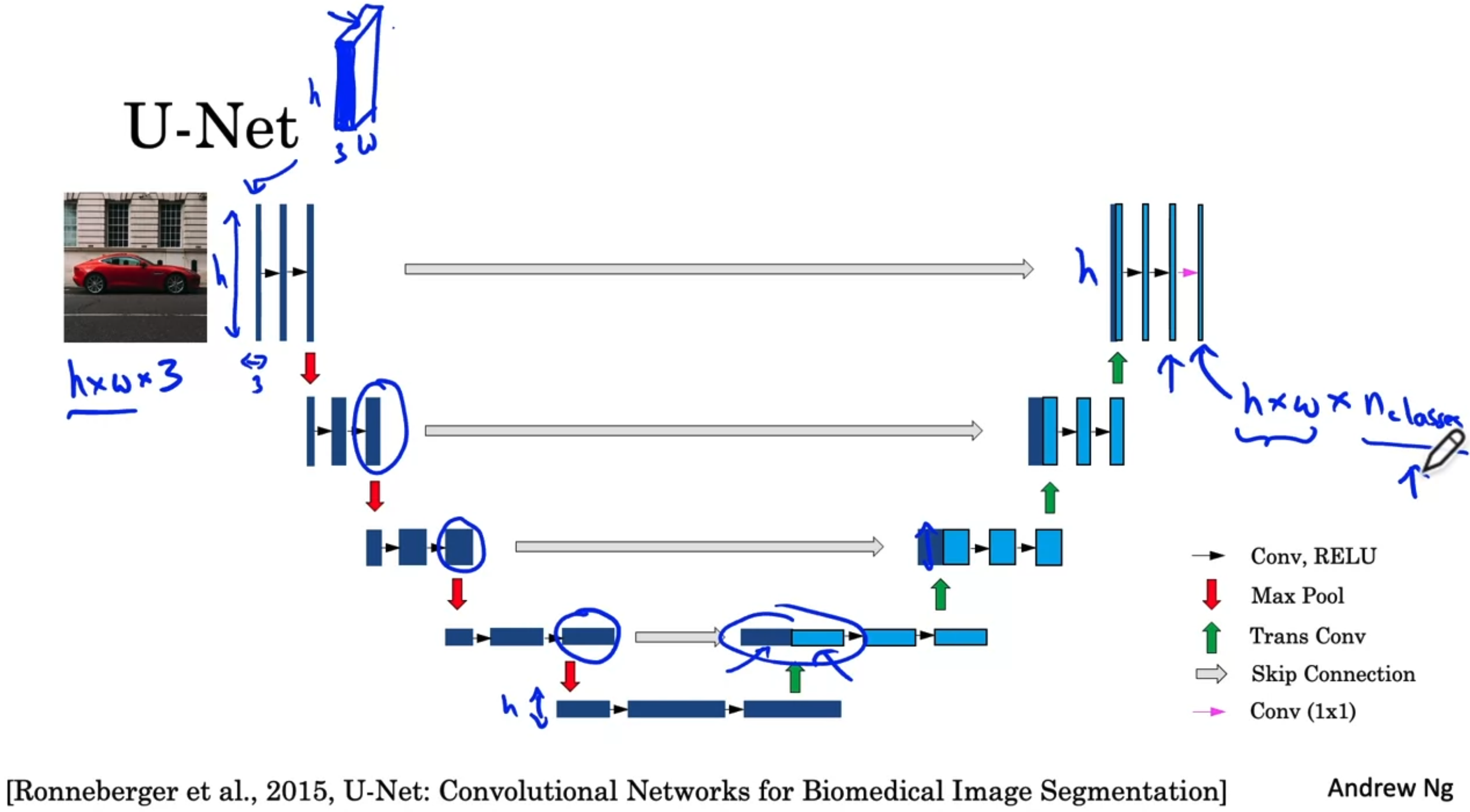
Semantic Segmentation with U-Net
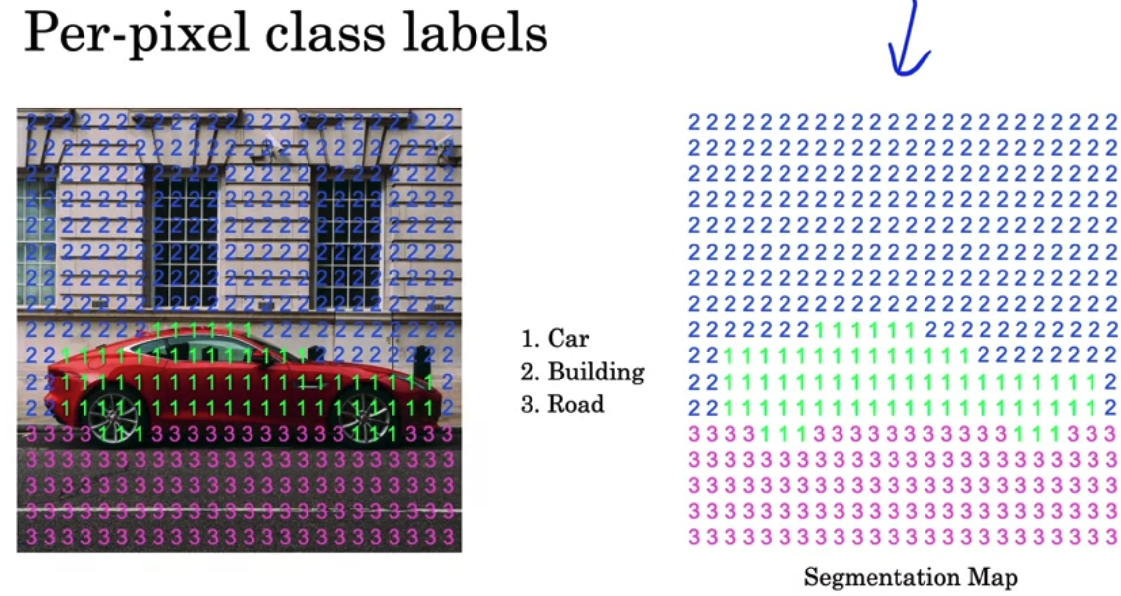
Per-pixel class labels
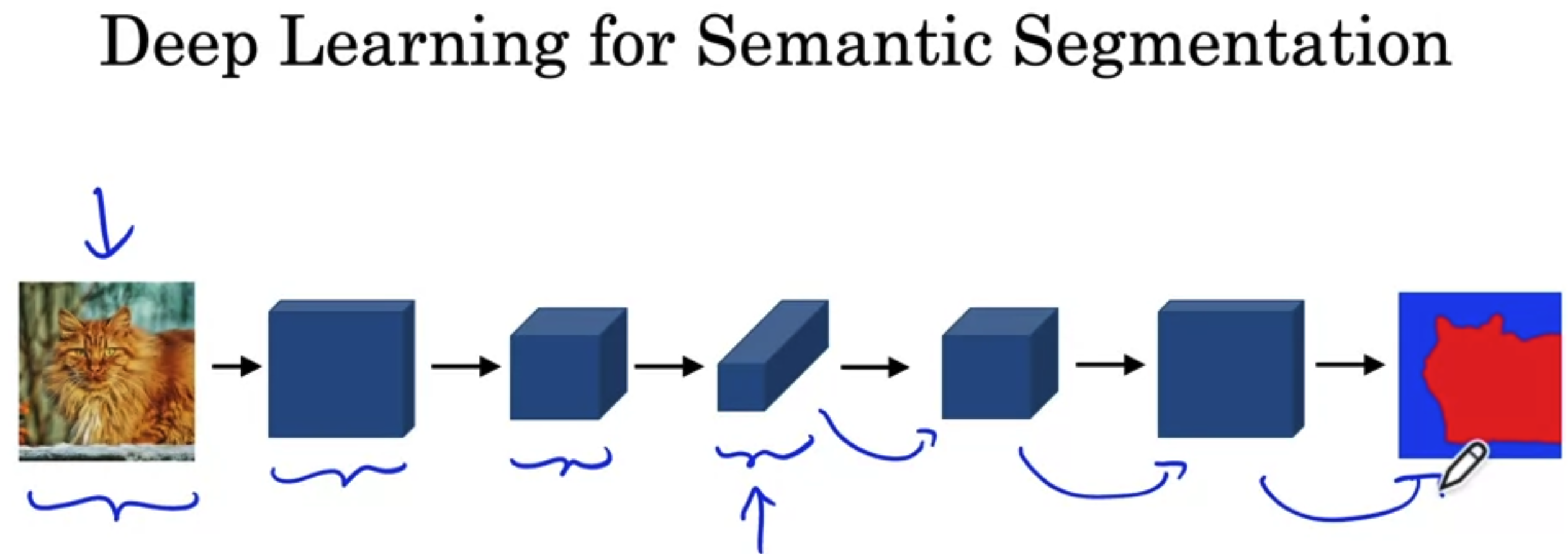
Deep Learning for Semantic Segmentation
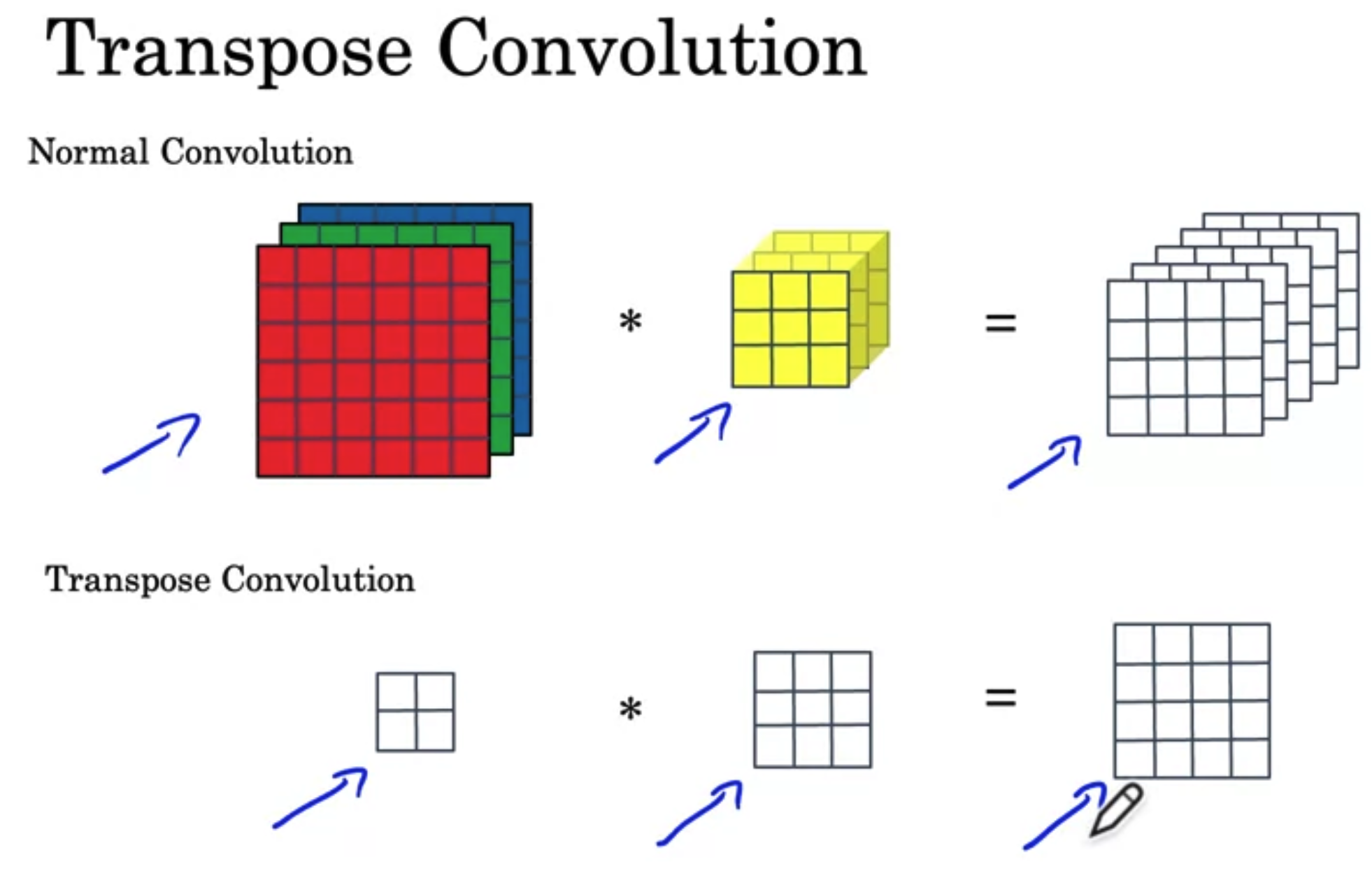
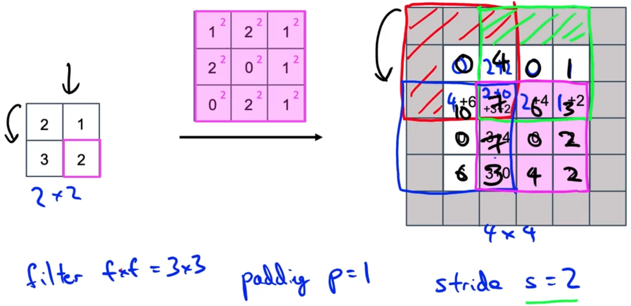
Transpose Convolution
- Increase the image size.
U-Net Architecture
- Skip Connections: Left one get more details in color or anything like that. Right one is more spatial information to figure out where is the object really is.
4.4 Special Applications: Face Recognition & Neural Style Transfer
4.4.1 Face recognition
Face verification vs. face recognition
- verification vs recognition —- 1:1 vs 1:K
- Verification
- Input image, name/ID.
- Output whether the input image is that of the claimed person.
- Recognition
- Has a database of K persons
- Get an input image
- Output ID if the image is any of the K persons (or “not recognized”)
One-shot learning
- Learning from one example to recognize the person again.
- Learning a “similarity” function
- d(img1, img2) = degree of difference between images
- If d(img1, img2) “same” “Different”
Siamese network
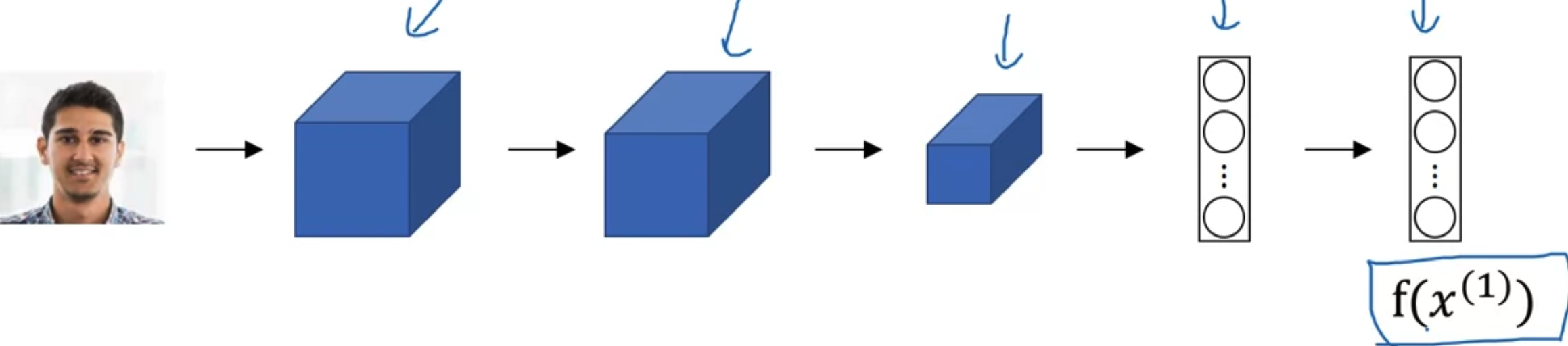
- Input two differnet images into two CNN and ge the result of them.
- Such as input seperately into two differnt CNN, and the output will be the encoding of each of them
- Then compare the distance between them
- Parameters of NN define an encoding
- Learn parameters so that:
- If are the smae person, is small.
- If are the different person, is large..
Triplet Loss
Learning objective: (Anchor, Positive), (Anchor, Negative)
- Want: is the margin (similar to SVM)
Loss function
- Given 3 images A, P, N:
If have a training set of 10K pictures of 1k persons. Put those 10K into triplet A, P, N, then put into the loss function.
Choosing the triplets A, P, N
- During training, if A, P, N are chosen randomly, is easily satisfied.
- Choose triplets that’re “hard” to train on. (such as choose )
Training set using triplet loss to make J smaller. And make distance of d for same person small and different large.
Face Verification and Binary Classification
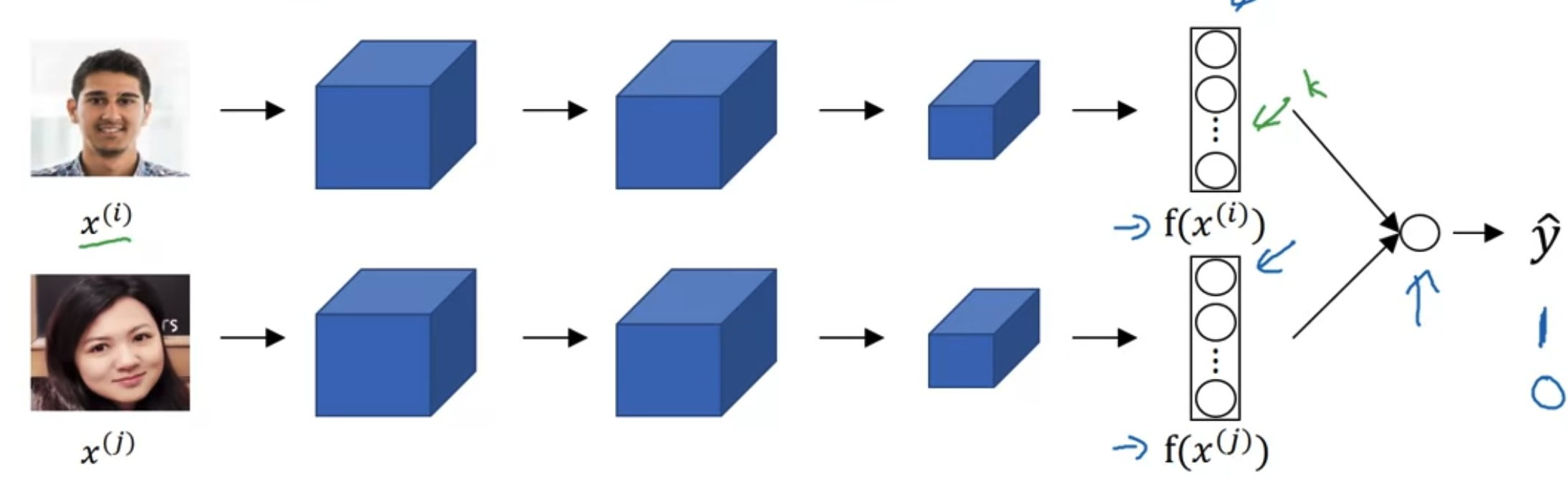
- Only store the as pre-compute, save storage and computational resources.
- Face verification supervised learning.
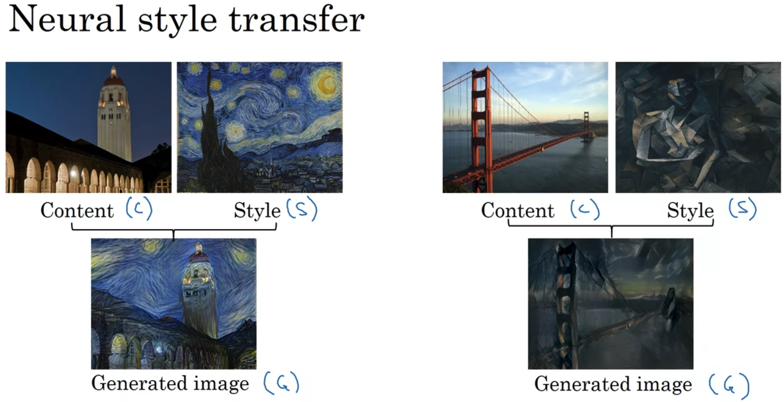
4.4.2 Neural style transfer
- What is it?
- Cost Function
- Find the generated image G
- Initiate G randomly G: 100x100x3
- Use gradient descent to minimize J(G)